
Sometimes query tuning involves taking a different approach to a problem. And given that other tuning options might be creating index(es) or redesigning tables – both of which are much more permanent changes to an environment – rewriting a query can often be just right.
Window functions seem to pop up quite often when rewriting queries, and an example around this would be appropriate for this month’s T-SQL Tuesday, hosted by Steve Jones (@way0utwest at X/Twitter).
One of the scenarios I loved when ranking functions first popped up was to use ROW_NUMBER() and a derived table to join adjacent rows. For example, suppose I want to look at adjacent rows in a temporal history table, the history of a table that has a primary key on the columns (pk1, pk2), using ValidFrom and ValidTo for its period. And suppose I want to look for where these adjacent rows are identical in the other columns, because maybe there’s been some updates to the main table, where rows have been updated without actually changing the data.
The table is simple, just this (options like collations, filegroups, compression have been removed to simplify the script)
[sql]create table dbo.SampleTemporalTable(
pk1 int not null,
pk2 nvarchar(255) not null,
val1 int null,
val2 varchar(10) null,
val3 date null,
ValidFrom datetime2 generated always as row start hidden,
ValidTo datetime2 generated always as row end hidden,
period for system_time(ValidFrom, ValidTo),
primary key clustered (pk1, pk2)
)
with (system_versioning=on (history_table = history.SampleTemporalTable));
drop index history.SampleTemporalTable.[ix_SampleTemporalTable];
create clustered index cix_history_SampleTemporalTable on history.SampleTemporalTable (pk1, pk2, ValidFrom, ValidTo);
[/sql]
I have included the script to drop the default clustered index and replace it with one that I find more useful. I always do this with temporal tables, but it’s particularly important for the performance I want today.
For my demo, I’ve got about 1200 rows in my main table, and about 6000 rows in my history table. Five identical copies of each row in my main table. I basically inserted the 1200 rows, and then updated a column without changing it (set val1 = val1) five times.
As for those adjacent rows, the way temporal history tables work is that each row has the same value in ValidFrom as in the previous version’s ValidTo, and there shouldn’t be two rows with the same values in (pk1, pk2, ValidFrom). I put ValidTo in my clustered index keys to help handle a situation where I do have clashes on (pk1, pk2, ValidFrom), but it shouldn’t happen naturally (only if the history table is being manipulated).
So this query should work, a simple join for when one row is replaced with another.
[sql]select *
from history.SampleTemporalTable thisrow
join history.SampleTemporalTable nextrow
on nextrow.pk1 = thisrow.pk1
and nextrow.pk2 = thisrow.pk2
and nextrow.ValidFrom = thisrow.ValidTo
where nextrow.val1 = thisrow.val1
and nextrow.val2 = thisrow.val2
and nextrow.val3 = thisrow.val3
;[/sql]
This isn’t too bad, except for handling potential NULL values in the columns val1, val2, val3, and that artificial situation where there could be multiple ValidFrom values. I’ll come back to that though, since right now I’m mostly interested in the execution plan.
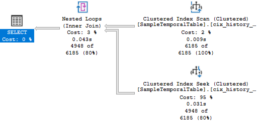
The plan for this query uses a Nested Loop, which pulls 6000 rows out of a Scan and calls a Seek for each of those rows. It’s not too bad, but it could definitely be better.
Lets jump into that ROW_NUMBER() with derived table option that I alluded to above. This method handles the situations when ValidFrom doesn’t match ValidTo – maybe a row was deleted for a while and then got reinserted – or that case where there are multiple rows with the same ValidFrom, by including ValidTo in the OVER clause’s ORDER BY. It’s a familiar pattern – I’ll use a CTE for my derived table.
[sql]with numberedrows as (
select *, row_number() over (partition by pk1, pk2 order by ValidFrom, ValidTo) as rownum
from history.SampleTemporalTable
)
select *
from numberedrows thisrow
join numberedrows nextrow
on nextrow.pk1 = thisrow.pk1
and nextrow.pk2 = thisrow.pk2
and nextrow.rownum = thisrow.rownum + 1
where nextrow.val1 = thisrow.val1
and nextrow.val2 = thisrow.val2
and nextrow.val3 = thisrow.val3
;[/sql]
This plan doesn’t use a Nested Loop – instead it has a Hash Match, and some operators to work out the ROW_NUMBER() value.

I not always a big fan of Hash Match joins. They definitely have their purposes, but I often find myself seeing what other options I have. The larger the number of rows, the larger the hash table in the Hash Match needs to be, so the memory needed grows with scale.
In this case, I feel like a Merge Join would be nicer. I have a clustered index designed to make sure the rows can be pulled in order. so this should be okay. I throw OPTION (MERGE JOIN) on the end, and look at the plan.
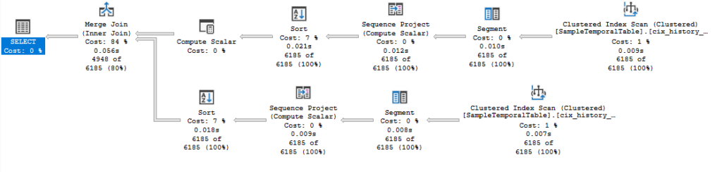
What?? A Sort? But I have the right clustered index for this, don’t I?
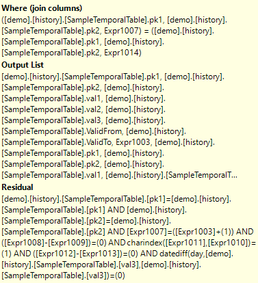
I investigate further, looking to see what we’re Sorting on, and the Join columns of the Merge Join.

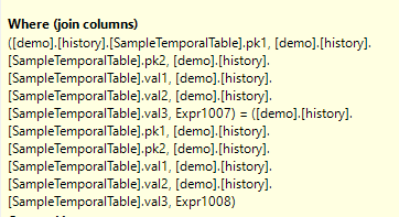
The Merge Join thinks that I want to join on all my columns! Not just the ones that I’m providing in the right order.
To be fair, I do only want to return the rows that match on val1, val2, and val3. So it’s correct – just not what I want for the best performance. It’s my own fault for trying to force it to use a Merge Join.
Before the real fix, let me show you what happens if I simply break the sargability on these additional predicates, to make them less amenable. And I mean really break. Not just using ISNULL() to handle the NULLs, which gives a similar plan, just with extra Compute Scalars.
No, when I break sargability, I really break it.
[sql]with numberedrows as (
select *, row_number() over (partition by pk1, pk2 order by ValidFrom, ValidTo) as rownum
from history.SampleTemporalTable
)
select *
from numberedrows thisrow
join numberedrows nextrow
on nextrow.pk1 = thisrow.pk1
and nextrow.pk2 = thisrow.pk2
and nextrow.rownum = thisrow.rownum + 1
/* Ugly non-sargable predicates here, to make sure they don’t get included in the Where property of the Merge Join) */
where isnull(nextrow.val1,-9999) – isnull(thisrow.val1,-9999) = 0
and charindex(isnull(nextrow.val2,’ZZZZ’),isnull(thisrow.val2,’ZZZZ’)) = 1
and len(isnull(nextrow.val2,’ZZZZ’)) – len(isnull(thisrow.val2,’ZZZZ’)) = 0
and datediff(day, nextrow.val3, thisrow.val3) = 0
option (merge join)
;[/sql]
Ugly, right?
I’m subtracting numbers from each other and seeing if it gives me zero. I’m comparing lengths and charindex of strings. And I’m doing a datediff for dates.
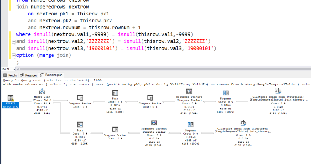
I’m really not suggesting you do this. But look at the plan change. It’s beautiful!

This is basically the plan that I wanted. The difference is in the properties of the Merge Join, where the Where columns are the PK values plus the rownum.
You see, Residuals aren’t always painful. You just need to understand when it’s appropriate to use them, and when it’s not.
Let’s solve this a better way though. One that’s been possible since SQL 2012.
I’m going to use LEAD. Across every column of the table. To make this code a little cleaner, I’m going to use a SQL 2022 feature, “WINDOW”, but for 2012-2019, just repeat the OVER clauses. This power of this method is going to be a subquery containing this block of code, which grabs everything from the next row without using ROW_NUMBER().
[sql]select pk1, pk2, val1, val2, val3, ValidFrom, ValidTo
, row_number() over win as rownum
, lead(val1) over win as val1_lead
, lead(val2) over win as val2_lead
, lead(val3) over win as val3_lead
, lead(ValidFrom) over win as ValidFrom_lead
, lead(ValidTo) over win as ValidTo_lead
from history.SampleTemporalTable
window win as (partition by pk1, pk2 order by ValidFrom, ValidTo)[/sql]
This gets to the lead values with a single pass of the data, and no extra Sort operators.

The inner workings of LEAD are interesting, but that’s another post. (The Aggregate operator on the left is pulling two rows from the Window Spool each time, and then combining them into one using an internal LAST_VALUE (even though we know that’s not an aggregate function). And it’s grouping by a “WindowCount” value.)
Anyway, using this subquery as a derived table gives me an easy way of checking the adjacent rows. I don’t need to break sargability any more, so I can just compare the values. And I’m going to use my preferred way of handing nulls, which is to use EXISTS and INTERSECT/EXISTS (rather than IS NOT DISTINCT FROM)
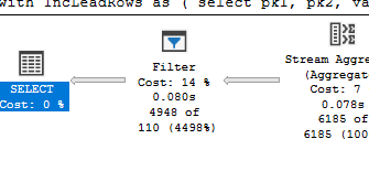
[sql]with IncLeadRows as (
select pk1, pk2, val1, val2, val3, ValidFrom, ValidTo
, row_number() over win as rownum
, lead(pk1) over win as pk1_lead
, lead(pk2) over win as pk2_lead
, lead(val1) over win as val1_lead
, lead(val2) over win as val2_lead
, lead(val3) over win as val3_lead
, lead(ValidFrom) over win as ValidFrom_lead
, lead(ValidTo) over win as ValidTo_lead
from history.SampleTemporalTable
window win as (partition by pk1, pk2 order by ValidFrom, ValidTo)
)
select *
from IncLeadRows
where exists (
select val1, val2, val3
intersect
select val1_lead, val2_lead, val3_lead
)
;[/sql]
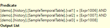
It simply adds a Filter operator on the left of the plan, but everything else is identical. A single scan of the data, with no Sort.
And that Filter? It’s nice and pure. Nothing to handle nulls at all. Because inside plans, null is just another value.
So now you know how I look for identical adjacent rows, and the kind of thing I look for in plans.
Comparing the estimated costs of those plans, I can see expect my new query is going to be significantly faster (estimated 17% to 83%, or about 5x cheaper). I’ll leave comparing the actual time using a much larger dataset to you if you’re interested. For me, I’m happy to feel like this plan is good, without having to use hints or do nasty non-sargable stuff.

Happy tuning…
@robfarley.com@bluesky (previously @rob_farley@twitter)
This Post Has 2 Comments
Hey Rob, Thanks for your valuable time and support for this article. Will see you on 29 Nov for Data Meetup at Adelaide.
Terrific. See you then.